
6. Seismic analysis: Difference between revisions
No edit summary |
No edit summary |
||
| Line 12: | Line 12: | ||
|- | |- | ||
|6.1 Short Term Seismic Hazard Assessment | |6.1 Short Term Seismic Hazard Assessment | ||
[[File:Short term seismic.png|150px|link=]] (Woodward 2015) | [[File:Short term seismic.png|150px|link=]] | ||
(Woodward 2015) | |||
|<li>Cumulative number of events chart</li> | |<li>Cumulative number of events chart</li> | ||
<li>Spatial plots to assess response extents</li> | <li>Spatial plots to assess response extents</li> | ||
| Line 32: | Line 33: | ||
|- | |- | ||
|6.4 Medium/Long Term Source Characterisation | |6.4 Medium/Long Term Source Characterisation | ||
[[File:Medium long term characterisatoin.png|150px|link=]] (Wesseloo et al. 2014) | [[File:Medium long term characterisatoin.png|150px|link=]] | ||
(Wesseloo et al. 2014) | |||
|<li>S:P energy ratio</li> | |<li>S:P energy ratio</li> | ||
<li>Moment tensor planes</li> | <li>Moment tensor planes</li> | ||
Revision as of 15:50, 15 August 2018
| Basic Practices | Advanced Properties | |
| 6.1 Short Term Seismic Hazard Assessment
|
||
| 6.2 Re-entry Analysis
|
||
| 6.3 Medium/Long Term Hazard Assessment
|
||
| 6.4 Medium/Long Term Source Characterisation
|
||
| 6.5 SGM Interpolation
|
The seismic analysis step is where the seismic data is used to assess the seismic hazard and to understand the sources of seismicity and response to mining. The assessment of seismic hazard is generally divided into analysis techniques for short term seismic responses (short term seismic hazard) and medium- to long-term seismic hazard assessment techniques. Seismic analysis is also used to investigate seismic sources and mechanisms to increase the understanding of the rock mass response to mining.
Short-term seismic hazard focuses on two components; namely:
- quantifying elelevated seismicity and its decay after blasts and large events, and, analysis of seismic responses often refered to as “Omori analysis”; and
- the detection of change in seismicity resulting in short term elevated seismic hazard, i.e time series analysis.
6.1 Short term seismic hazard assessment
6.1.1 Basic
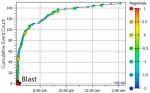
For the analysis of seismic responses after blasts and large events, the basic approaches include the qualitative assessment of a time series chart (e.g. magnitude-time, daily histogram, cumulative event count) and spatial plot of seismicity (e.g. plan view, 3D view). This style of analysis is done on the vast majority of sites irrespective whether more advanced approaches are also considered. The following figure provides an example of a seismic response to a large event. Spatial plot is shown left and an annotated time series is shown right (Vallejos and McKinnon 2010).
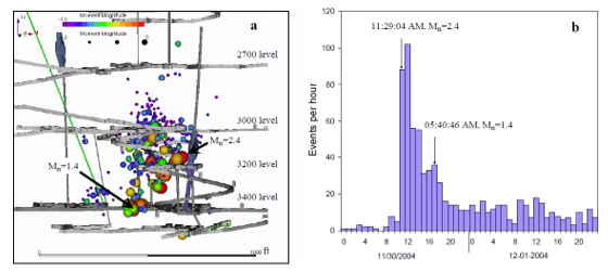
Figure: A spatial plot a) and cumulative event count time series b) for a seismic response to a large seismic event (Vallejos and McKinnon 2010)
Additionally, the time of day of events is commonly used to evaluate to what degree seismicity is related to blasting; specifically, to estimate the rate of seismicity that occurs independent of blasting (background rate). The figure below provides an example of a diurnal chart (Vallejos and McKinnon 2010).
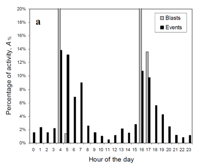
Figure: Diurnal chart of seismic and blast activity (Vallejos and McKinnon 2010)
6.1.2 Advanced
Advanced analysis of seismic responses incorporates seismic source parameters into the assessment and/or aims to quantify the space-time characteristics of a response. Temporal assessment of seismic responses can incorporate the location of events by defining an analysis volume. These are arbitrary volumes often defined by coordinates, as shown in the following figure, or by only considering events within a certain distance from a blast.
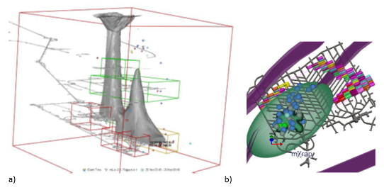
Figure: Spatial volumes (green frames/polygons) are defined with respect to mine surveys a) or elipsoids around blast locations b) to intoduce a spatial component to temporal analysis
The most common method of incorporating seismic source parameters is to consider a rate or accumulation of a parameter value over time.
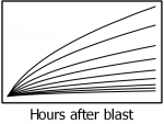
Advanced analysis also aims to quantify seismic responses by fitting a temporal model to event occurrence. This model is most commonly the Modified Omori Law (MOL) which was derived from the study of earthquake aftershocks (Omori 1894); for example, the following figure shows the MOL which models five responses to blasting (Plenkers et al. 2010). Temporal modelling approaches incorporate the location of events by either considering arbitrary areas of a mine, volumes around blasts, clusters determined visually, or clustered determined by an algorithm.
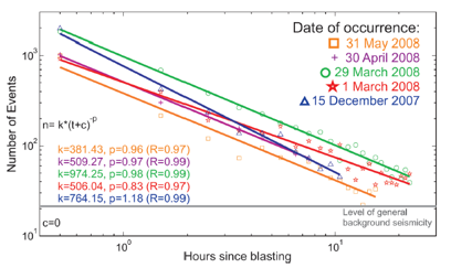
Figure: Application of the MOL to seismic responses following blasting. Seismic event rate is plotted with respect to the fitted model and background rate of seismicity (Plenkers et al. 2010)
Time series analysis aims at detecting anomalous seismic behaviour as a precursor to elevated seismic hazard. These types of assessments are often used in conjunction with each other. One of the most common approaches is to examine energy-index and cumulative apparent volume, Schmidt Number and extraction induced seismic strain, over time, as shown in the following two figures. Other approaches include cumulative energy, apparent stress time history, ratio of s-wave energy to p-wave energy, static stress drop, and dynamic stress drop.
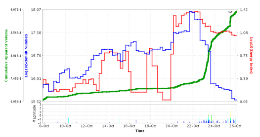
Figure: Time history of CAV, EI and Scs for about one month before a m 1.2 at a deep gold mine in South Africa (Rebuli and van Aswegen 2013)
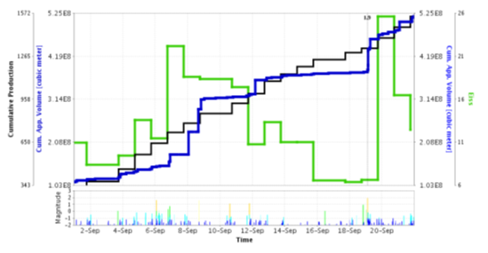
Figure: Time history of CAV, cumulative production and EISSr for about one month before a m 1.9. EISSr shows a steady drop a few days before the m 1.9 event (Rebuli and van Aswegen 2013)
6.2 Re-entry analysis
6.2.1 Basic
The topic of re-entry is covered in two sections. This section focuses on the analysis of data following blasts and large events and the derivation of rules. The application of these rules and real-time monitoring of seismicity and re-entry decisions is discussed under the Control section (10.1.2). For many sites, re-entry protocols are not based on back analysis of seismicity, but rather on choosing conservative re-entry periods. Some sites with enough flexibility in the mining schedule allow long periods before re-entry by sheduling work to be performed in areas further away from recent blasts.
6.2.2 Advanced
Re-entry analysis uses short-term assessment techniques to characterise current and/or historical seismic responses. Blanket exclusion rules are developed from historical responses and consider practical operational constraints. These rules are typically conservative by design and use the assessment of a current seismic response to refined exclusions. Cumulative event count: count of the events that occur within a fixed analysis period (e.g. six hours after) and distance (e.g. 50 m) from blast. Re-entry protocol length is based on an arbitrary event percentage for historical responses; for example, protocols are lifted when 90% of events occurred for historical responses.
Seismic event rate – Return to background: re-entry protocols are lifted when the rate of seismicity returns to a previously determined background rate. This is evaluated in several ways ranging from qualitative assessment (e.g. when the slope of cumulative events looks similar to that prior to the blast) to quantitative assessment. IMS STAT is an example where such analysis is performed in real time and translated to a traffic light system for real-time assessment for re-entry times.
6.3 Medium/long term hazard assessment
6.3.1 Basic
Seismic hazard over the longer term is generally reported using simple statistics. Weekly and monthly reports usually include the total number of events recorded, as well as the number of large/significant events. Sometimes the event count over the previous reporting periods is included for reference.
The cumulative number of events is usually used to assess changes in seismic activity rate over time; higher gradients generally representing periods of elevated hazard. The areas within the mine with elevated hazard are often evaluated with event density plots. Event density isosurfaces, as demonstrated in the figure below, are plotted based on an event count within a certain radius. Sometimes a threshold event magnitude is applied to the event count to reduce the effect of varying seismic system sensitivity across the mine.
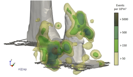
Figure: Example of a seismic event density plot
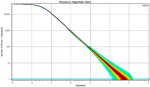
The following figure is a frequency-magnitude chart and is used to quantify and visualise the size distribution of events. Many operations use the magnitude where the Gutenberg–Richter relationship at N = 1 (sometimes referred to as the a/b value) as an estimate of medium/long term hazard although in some cases there might not be a sufficient appreciation of the importance of accounting for scale effects in both space and time.
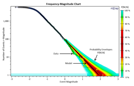
Figure: Example frequency–magnitude chart, Gutenberg–Richter distribution and probabilistic hazard
Another basic approach to seismic hazard assessment is to use a simple linguistic scale. The Seismic Hazard Scale in the table below uses a derivation of the Gutenberg–Richter relationship to represent the seismic hazard in terms of a single Richter magnitude seismic event or a qualitative description. The Rosebery mine uses an adapted form of the Seismic Hazard Scale to track seismic hazard. The qualitative description of the scale is used to communicate the seismic hazard more effectively with underground personnel and mine management.
| Seismic Hazard Scale (SHS) defined from daily rates of seismic events and qualitative event descriptions | ||||||
| Mine seismicity frequency per day | ||||||
| Qualitative description | Felt locally | Felt in a few parts of a mine, like a secondary blast | Often felt on surface, or like a development blast | Felt like a production mass blast | Detected by regional earthquake network | |
| Approx. Richter magnitude | ML >= -2 | ML >= -1 | ML >= 0 | ML >= +1 | ML >= +2 | |
| Seismic hazard scale and qualitative description | ||||||
| -2 | Nil | >0.001 (once every few years) | 0 (has never occurred) | 0 (has never occurred) | 0 (has never occurred) | 0 (has never occurred) |
| -1 | Very low | >0.01 (a few times per year) | >0.001 (once every few years) | 0 (has never occurred) | 0 (has never occurred) | 0 (has never occurred) |
| 0 | Low | >0.1 (at least weekly) | >0.01 (a few times per year) | >0.001 (once every few years) | 0 (has never occurred) | 0 (has never occurred) |
| 0.5 | Low to moderate | >0.3 (a few times per week) | >0.03 (monthly) | >0.003 (yearly) | <0.001 (may have happened once) | 0 (has never occurred) |
| 1 | Moderate | >1 (at least daily) | >0.1 (at least weekly) | >0.01 (a few times a year) | >0.001 (once every few years) | 0 (has never occurred) |
| 1.5 | Moderate to high | >3 (a few a day) | >0.3 (a few times a week) | >0.03 (monthly) | >0.003 (yearly) | >0.001 (may have happened once) |
| 2 | High | >10 (more than 10 a day) | >1 (at least daily) | >0.1 (at least weekly) | >0.01 (a few times a year) | >0.001 (once every few years) |
| 2.5 | High to very high | >30 (more than 30 a day) | >3 (a few a day) | >0.3 (a few times a week) | >0.03 (monthly) | >0.003 (yearly) |
| 3 | Very high | >100 (more than 100 a day) | >10 (more than 10 a day) | >1 (at least daily) | >0.1 (at least weekly) | >0.01 (a few times a year) |
| 3.5 | Very high to extreme | >300 (more than 300 a day) | >30 (more than 30 a day) | >3 (a few a day) | >0.3 (a few times a week) | >0.03 (monthly) |
| 4 | Extreme | >1000 (more than 1000 a day) | >100 (more than 100 a day) | >10 (more than 10 per day) | >1 (at least daily) | >0.1 (at least weekly) |
Table: Qualitative seismic hazard scale (Hudyma and Potvin 2004)
6.3.2 Advanced
Although the investigation into pre-cursors to earthquakes and mining-induced seismic events are continuing, it is well recognised that meaningful predictions of large seismic seismic events are not currently possible. Given the inherent variability and uncertainty of mine seismicity, results from advanced seismic hazard assessments are often probabilistic (see figure below).
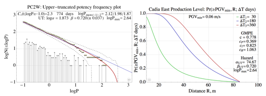
Figure: a) Size distribution plot and the observed (blue dots) and theoretical (solid red) distribution for a section of the mine; b) Probability that PGV >= 0.06 m/s will occur for a section of the mine (after Mendecki 2017)
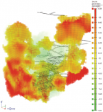
Some form of probabilistic seismic hazard (PSHA) is now increasingly used in the industry with 87% of online survey responders saying they have used the grid-based PSHA as shown in the following figure within the last 12 months. The grid-based hazard assessment quantifies the current hazard state based on the recent historical data. Seismic hazard is calculated probabilistically and expressed as hazard ratings and as probabilistic hazard maps.
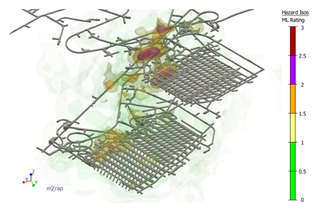
Figure: Example grid-based PSHA map at the Cadia Valley Operation
The seismic hazard for mine development is often expressed as the probability of exceeding a design peak particle velocity (PPV) within a defined time period. The estimation of seismic hazard in terms of PPV requires a site ground motion prediction equation (GMPE) to calculate the magnitude of the ground motion based on the distance and seismic event source parameters, as demonstrated in the figure below.
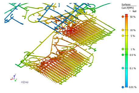
Figure: Example PPV hazard map at the Cadia Valley Operation mine
The PPV map in the above figure uses the grid-based results to perform the probabilistic evaluation of PPV’s on the development. This approach estimates the current seismic hazard based on recently recorded data. The Peak Ground Velocity (PGV) map (note that PPV and PGV is the same) in the below figure incorporates modelling information to estimate ground motions for the future mining geometry.
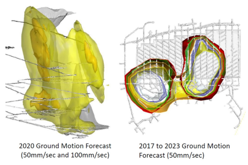
Figure: PGV maps from Salamon-Linkov modelling
6.4 Medium/long term source characterisation
6.4.1 Basic
It is important for the site geotechnical team to form an appreciation of the different sources of seismicity in the mine, their characteristics and their likely responses to mining activity. This appreciation is obtained through back analysis and detailed investigation into the recorded seismic and non-seismic data, interpreting different source parameters within the context of mining. In spite of its importance, this is not commonly done.
Some operations use the S:P energy ratio as an indication of seismic mechanism. High ratios, in theory, indicate a stronger shearing/deviatoric mechanism while lower ratios indicate a more crushing/ bursting/isotropic mechanism. Recent research has raised some doubt over the reliability of the S:P energy ratio parameter (Morkel et al. 2017).
6.4.2 Advanced
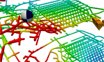
Methods used for medium/long term characterisation of seismic sources analyse seismic data in order to gain insight into the rock mass response to mining; either causation or mechanism of rock mass deformation. The use of moment tensor solutions is becoming more common but, based on the survey conducted, this is only done on an event-by-event basis. Generally, the fault plane of the moment tensor solution is compared with nearby geological orientations. It is less common for operations to use the moment tensor decomposition.
Volume/Polygon-based assessments of source parameters are sometimes performed to quantify the rock mass behaviour in a specified volume. The evaluation of Energy index (EI) and Apparent stress is often used as an indicator of stress, cumulative apparent volume, or the cube root of moment as an indicator of co-seismic rock mass strain and b-value as an indicator of fracture mechanism.
Grid-based analysis is becoming more popular as a seismic analysis tool and is being used by 87% of survey responders. The grid-based approach does not rely on user-chosen analysis volumes and is free of bias due to user-decision on volume selection. It still requires user input, so it is not free of user influence.
An example of a grid-based approach is shown in the figure below which shows the results of grid-based analysis of the Energy Index (EI) and Seismic Displacement parameters. In this case, EI is used as a proxy for the stress state of the rock mass and the seismic displacement used as a proxy for damage. This analysis provides valuable indications as to the state of the rock mass and the response to mining activity.
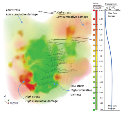
Figure: Grid-based analysis of EI and Seismic Displacement (Wesseloo et al. 2014)
6.5 SGM interpolation
6.5.1 Basic
Strong ground motion (PPV or PPA) is often used as a parameter for seismic hazard intensity. The derivation of site-specific relationships is required. This is becoming more common, but is not performed on all sites, with some sites using generic relationships presented in literature. Using the strong ground motion relationship and the properties of an event, the theoretical strong ground motion experienced at an excavation is often calculated to assess the effect of large remote events on excavation, as demonstrated in the following figure.
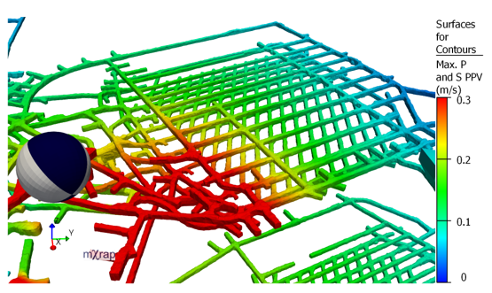
Figure: Theoretical experienced ppv ground motion experienced
6.5.2 Advanced
Advanced practice includes regular updates of the strong ground motion relationship. Interpolation of the strong ground motion on a real time basis is currently under development and shows promise as a monitoring tool for the purpose of triggering an action.