
5. Numerical models: Difference between revisions
No edit summary |
No edit summary |
||
| (16 intermediate revisions by 3 users not shown) | |||
| Line 1: | Line 1: | ||
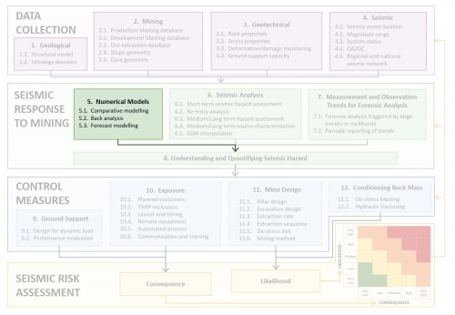
__NOTOC__ | |||
[[File: | [[File:2.05_Numerical_Models.jpg|500px|left|link=]] | ||
<br clear=all> | |||
{| class="wikitable" | {| class="wikitable" | ||
|- | |- | ||
| | | | ||
| | |Standard Practices | ||
|Advanced Properties | |Advanced Properties | ||
|- | |- | ||
|5.1 Comparative Modelling | |5.1 Comparative Modelling | ||
[[File:Comparative modelling.png| | [[File:Comparative modelling.png|150px|link=]] | ||
|<li>Compare shear stress on major structures for different extraction sequences using 3D elastic model | |<li>Compare shear stress on major structures for different extraction sequences using 3D elastic model | ||
<li>Assess stress/energy/displacement criteria for different excavation arrangements | <li>Assess stress/energy/displacement criteria for different excavation arrangements | ||
|<li>Compare anticipated seismic | |<li>Compare anticipated seismic responses for different sequences | ||
<li>Assess the effect of different loading sequences on the rock mass and exposure of work areas based on variations in mine design | <li>Assess the effect of different loading sequences on the rock mass and exposure of work areas based on variations in mine design | ||
|- | |- | ||
|5.2 Back Analysis | |5.2 Back Analysis | ||
[[File:Back analysis.png| | [[File:Back analysis.png|150px|link=]] | ||
|<li>Review stress conditions leading up to previous large events | |<li>Review stress conditions leading up to previous large events | ||
<li>Consider whether observed rock mass behaviour matches expectations, review input parameters if necessary | <li>Consider whether observed rock mass behaviour matches expectations, review input parameters if necessary | ||
| Line 24: | Line 26: | ||
|- | |- | ||
|5.3 Forecast Modelling | |5.3 Forecast Modelling | ||
[[File:Forecast modelling 1.png| | [[File:Forecast modelling 1.png|60px|link=]] [[File:Forecast modelling 2.png|60px|left=]] | ||
|<li>Use established correlations to assess potential conditions as mining progresses | |<li>Use established correlations to assess potential conditions as mining progresses | ||
<li>Identify trigger levels in model results that correlate to observed behaviour | <li>Identify trigger levels in model results that correlate to observed behaviour | ||
| Line 32: | Line 34: | ||
== 5.1 Comparative modelling == | == 5.1 Comparative modelling == | ||
Numerical modelling, in conjunction with data analysis and interpretation, plays an important role in the management of seismic risk. Numerical modelling provides a “laboratory” for testing different “what if?” scenarios and assessing possible rock mass behaviour for these different scenarios. Numerical modelling constitutes a wide range of approaches, different software and different levels of complexity. These different approaches, software and complexity levels can all be used effectively, but a clear distinction should be made between calibrated and uncalibrated models. | Numerical modelling, in conjunction with data analysis and interpretation, plays an important role in the management of seismic risk. Numerical modelling provides a “laboratory” for testing different “what if?” scenarios and assessing possible rock mass behaviour for these different scenarios. Numerical modelling constitutes a wide range of approaches, different software and different levels of complexity. These different approaches, software and complexity levels can all be used effectively, but a clear distinction should be made between calibrated and uncalibrated models. | ||
| Line 41: | Line 41: | ||
Best practice in numerical modelling should be judged on the level of calibration to observation rather than any particular approach or software used. | Best practice in numerical modelling should be judged on the level of calibration to observation rather than any particular approach or software used. | ||
Another important distinction that needs to be made is the appropriate scale at which the modelling results need to be interpreted. Some sites have reported a good correlation between modelled and experienced behaviour at a mine- wide scale, but a poor correlation at drive scale. This concept of scale-appropriate modelling is illustrated by Levkovitch et al. (2008) in | Another important distinction that needs to be made is the appropriate scale at which the modelling results need to be interpreted. Some sites have reported a good correlation between modelled and experienced behaviour at a mine-wide scale, but a poor correlation at drive scale. This concept of scale-appropriate modelling is illustrated by Levkovitch et al. (2008) in the following figure. | ||
[[File:Figure 26.png| | [[File:Figure 26.png|link=]] | ||
Figure | Figure: A guide to the method of including discontinuities of different length scales in a geotechnical numerical model, based on the scale of the phenomena that are being targeted (Levkovitch et al. 2008) | ||
The use of numerical modelling varies significantly in the industry, with some sites relying heavily on mine-wide calibrated elasto-plastic models for the purpose of seismic hazard assessment, while others do not incorporate numerical modelling directly into their systems for managing seismic hazard. | The use of numerical modelling varies significantly in the industry, with some sites relying heavily on mine-wide calibrated elasto-plastic models for the purpose of seismic hazard assessment, while others do not incorporate numerical modelling directly into their systems for managing seismic hazard. | ||
=== 5.1.1 | === 5.1.1 Standard === | ||
Standard comparative models often rely on elastic modelling and/or modelling of an elastic rock mass with elasto-plastic faults, and/or dykes (generally performed with Map3D). Criteria for the comparison of these models include: | |||
<ul> | <ul> | ||
| Line 58: | Line 58: | ||
<li>excess shear stress;</li> | <li>excess shear stress;</li> | ||
<li>energy release rate;</li> | <li>energy release rate;</li> | ||
<li> | <li>remnant failure index; and</li> | ||
<li> | <li>local energy release rate (LERR).</li> | ||
</ul> | </ul> | ||
| Line 66: | Line 66: | ||
=== 5.1.2 Advanced === | === 5.1.2 Advanced === | ||
Comparative models are also performed in more sophisticated analysis approaches where both the rock mass and faults or dykes are modelled as an elasto-plastic material. An example of such an approach is the comparison of potential seismic moment (proportional to modelled shear slip) on fault for different scenarios (Sjöberg et al. 2012) | Comparative models are also performed in more sophisticated analysis approaches where both the rock mass and faults or dykes are modelled as an elasto-plastic material. An example of such an approach is the comparison of potential seismic moment (proportional to modelled shear slip) on fault for different scenarios (Sjöberg et al. 2012), as shown in the figure below. | ||
[[File:Figure 27.png| | [[File:Figure 27.png|link=]] | ||
Figure | Figure: Calculated seismic moment in NM for all structures and for future mining according to Case 1 and 2 (Sjöberg et al. 2012) | ||
A considerable range of sophistication exists in the elasto-plastic material models; from simpler elastic-perfectly plastic and elastic-perfectly brittle to the more sophisticated models with strain hardening/softening behaviour and stress dependent dilatational behaviour. Therefore, different criteria are used for comparative models. | A considerable range of sophistication exists in the elasto-plastic material models; from simpler elastic-perfectly plastic and elastic-perfectly brittle to the more sophisticated models with strain hardening/softening behaviour and stress dependent dilatational behaviour. Therefore, different criteria are used for comparative models. | ||
Recently, a modelling approach incorporating the Salamon-Linkov model into a boundary element approach has been developed by Dr. Dmitri Malovichko (Malovichko 2017). At a fundamental level, this modelling approach differs from elasto-plastic approaches as it explicitly incorporates the modelling of seismic events occurrence rather than correlating seismic potential with parameters of elastic modelling | Recently, a modelling approach incorporating the Salamon-Linkov model into a boundary element approach has been developed by Dr. Dmitri Malovichko (Malovichko 2017). At a fundamental level, this modelling approach differs from elasto-plastic approaches as it explicitly incorporates the modelling of seismic events occurrence rather than correlating seismic potential with parameters of elastic modelling, as shown in the figure below. | ||
[[File:Figure 28.png| | [[File:Figure 28.png|link=]] | ||
Figure | Figure: Results of modelling of expected seismicity using the Salamon-Linkov model (Malovichko 2017) | ||
Some of the surveyed sites performed modelling of dynamic wave-excavation interaction as input to support design. Such modelling does not provide insight into the seismic hazard assessment, but provides insight into the dynamic load experienced at an excavation, given that a specified seismic event occurs. | Some of the surveyed sites performed modelling of dynamic wave-excavation interaction as input to support design. Such modelling does not provide insight into the seismic hazard assessment, but provides insight into the dynamic load experienced at an excavation, given that a specified seismic event occurs. The following figure demonstrates results of dynamic wave modelling and indicates the wave–excavation interaction. | ||
[[File:Figure 29.png| | [[File:Figure 29.png|link=]] | ||
Figure | Figure: a) Snapshots of a 2D section of the 3D wave field induced by the synthetic Ortlepp shear event (Mendecki and Lötter 2011); and b) Snapshots of velocity field (Wang and Cai 2015) | ||
== 5.2 Back analysis == | == 5.2 Back analysis == | ||
=== 5.2.1 | === 5.2.1 Standard === | ||
Back analysis of significant events is sometimes performed to provide a better understanding of the conditions leading to significant seismic events or rockbursts. A high mining-induced stress to strength ratio is often used as a criteria for back analysis where such zones are correlated with zones of elevated seismicity. | Back analysis of significant events is sometimes performed to provide a better understanding of the conditions leading to significant seismic events or rockbursts. A high mining-induced stress to strength ratio is often used as a criteria for back analysis where such zones are correlated with zones of elevated seismicity. | ||
| Line 95: | Line 95: | ||
Some of the criteria mentioned in Section 5.1.1 are back calculated parameters from seismic responses experienced in the past. This includes the back calculation of parameters for the ESS to match an experienced fault slip event and the back calculation of the average pillar stress at failure. | Some of the criteria mentioned in Section 5.1.1 are back calculated parameters from seismic responses experienced in the past. This includes the back calculation of parameters for the ESS to match an experienced fault slip event and the back calculation of the average pillar stress at failure. | ||
Stress and strain conditions in three-dimensional elasto-plastic analysis are also used to assess the conditions leading up to large events as illustrated in | Stress and strain conditions in three-dimensional elasto-plastic analysis are also used to assess the conditions leading up to large events as illustrated in the figure below (Kalenchuk et al. 2017). | ||
[[File:Figure 30.png| | [[File:Figure 30.png|link=]] | ||
Figure | Figure: Evolution of numerically predicted stresses leading up to the MN3.2 event and numerically predicted pillar yield (Kalenchuk et al. 2017) | ||
Some sites have sophisticated mine scale models that are updated and for which the calibration is improved from time to time. Such models provide a good opportunity to investigate what conditions lead up to large events or rockbursts. They also provide a good opportunity to back calculate parameter levels which can be used as values to flag possible adverse behaviour when using such models in forecast modelling. | Some sites have sophisticated mine scale models that are updated and for which the calibration is improved from time to time. Such models provide a good opportunity to investigate what conditions lead up to large events or rockbursts. They also provide a good opportunity to back calculate parameter levels which can be used as values to flag possible adverse behaviour when using such models in forecast modelling. | ||
Detailed forensic models are also run to obtain a better understanding of the mechanisms driving large events (Counter 2014) | Detailed forensic models are also run to obtain a better understanding of the mechanisms driving large events (Counter 2014), as shown in the figure below. | ||
[[File:Figure 31.png| | [[File:Figure 31.png|link=]] | ||
Figure | Figure: Forensic 3D elasto plastic model of a Mn3.9 seismic event. The slip surface is defined by major change in vector orientation and magnitude in the centre of the image. Local effect of unclamping in the foot wall caused by mining of a stope in the satallite lense (Counter 2014) | ||
== 5.3 Forecast modelling == | == 5.3 Forecast modelling == | ||
=== 5.3.1 | === 5.3.1 Standard === | ||
Some | Some standard modelling approaches with established correlations and back calculated trigger values are used in forecast modelling to flag future adverse scenarios. For example, correlation of high mining induced stress/strength ratio and elevated seismicity with back calculated trigger levels are used to forecast when and where in the mine life stress conditions leading to adverse seismicity is expected to occur. Similar forecast models are performed with other parameters mentioned in Section 5.1.1. | ||
=== 5.3.2 Advanced === | === 5.3.2 Advanced === | ||
Forecast modelling using mine-wide calibrated elasto-plastic modelling | Forecast modelling using mine-wide calibrated elasto-plastic modelling, as shown in the following figure, or Salamon-Linkov modelling is performed at some sites. Considerable time and effort is invested in these models as they need to periodically be updated and re-calibrated as new information becomes available. | ||
[[File:Figure 32.png| | [[File:Figure 32.png|link=]] | ||
Figure | Figure: Contours of plastic shear strain from elasto–plastic modeling with strain-softening material behaviour. Red approximates a jump in damage from minor to moderate, moderate to significant, or significant to very significant | ||
Latest revision as of 15:03, 10 May 2019
| Standard Practices | Advanced Properties | |
| 5.1 Comparative Modelling
|
||
| 5.2 Back Analysis
|
||
| 5.3 Forecast Modelling
|


5.1 Comparative modelling
Numerical modelling, in conjunction with data analysis and interpretation, plays an important role in the management of seismic risk. Numerical modelling provides a “laboratory” for testing different “what if?” scenarios and assessing possible rock mass behaviour for these different scenarios. Numerical modelling constitutes a wide range of approaches, different software and different levels of complexity. These different approaches, software and complexity levels can all be used effectively, but a clear distinction should be made between calibrated and uncalibrated models.
Uncalibrated models can be used for scenario comparisons, while calibrated models can be used for forecasting of expected future rock mass behaviour. Uncalibrated models are used to compare different scenarios to choose the most favourable among several possible options. In such cases, the decision is based on simple criteria that are assessed for the different scenarios.
Best practice in numerical modelling should be judged on the level of calibration to observation rather than any particular approach or software used.
Another important distinction that needs to be made is the appropriate scale at which the modelling results need to be interpreted. Some sites have reported a good correlation between modelled and experienced behaviour at a mine-wide scale, but a poor correlation at drive scale. This concept of scale-appropriate modelling is illustrated by Levkovitch et al. (2008) in the following figure.
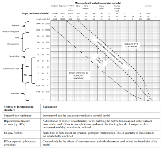
Figure: A guide to the method of including discontinuities of different length scales in a geotechnical numerical model, based on the scale of the phenomena that are being targeted (Levkovitch et al. 2008)
The use of numerical modelling varies significantly in the industry, with some sites relying heavily on mine-wide calibrated elasto-plastic models for the purpose of seismic hazard assessment, while others do not incorporate numerical modelling directly into their systems for managing seismic hazard.
5.1.1 Standard
Standard comparative models often rely on elastic modelling and/or modelling of an elastic rock mass with elasto-plastic faults, and/or dykes (generally performed with Map3D). Criteria for the comparison of these models include:
- stress to strength ratio in different areas of the mine;
- increase in mining-induced stress on a specific pillar of fault;
- excess shear stress;
- energy release rate;
- remnant failure index; and
- local energy release rate (LERR).
More details on these methods can be found in the recommended readings at the end of this document.
5.1.2 Advanced
Comparative models are also performed in more sophisticated analysis approaches where both the rock mass and faults or dykes are modelled as an elasto-plastic material. An example of such an approach is the comparison of potential seismic moment (proportional to modelled shear slip) on fault for different scenarios (Sjöberg et al. 2012), as shown in the figure below.
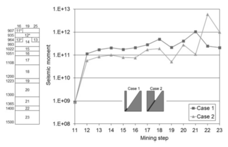
Figure: Calculated seismic moment in NM for all structures and for future mining according to Case 1 and 2 (Sjöberg et al. 2012)
A considerable range of sophistication exists in the elasto-plastic material models; from simpler elastic-perfectly plastic and elastic-perfectly brittle to the more sophisticated models with strain hardening/softening behaviour and stress dependent dilatational behaviour. Therefore, different criteria are used for comparative models.
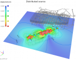
Recently, a modelling approach incorporating the Salamon-Linkov model into a boundary element approach has been developed by Dr. Dmitri Malovichko (Malovichko 2017). At a fundamental level, this modelling approach differs from elasto-plastic approaches as it explicitly incorporates the modelling of seismic events occurrence rather than correlating seismic potential with parameters of elastic modelling, as shown in the figure below.
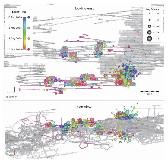
Figure: Results of modelling of expected seismicity using the Salamon-Linkov model (Malovichko 2017)
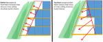
Some of the surveyed sites performed modelling of dynamic wave-excavation interaction as input to support design. Such modelling does not provide insight into the seismic hazard assessment, but provides insight into the dynamic load experienced at an excavation, given that a specified seismic event occurs. The following figure demonstrates results of dynamic wave modelling and indicates the wave–excavation interaction.
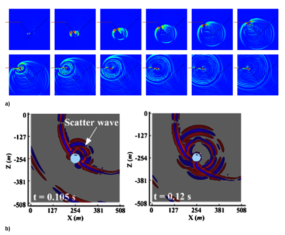
Figure: a) Snapshots of a 2D section of the 3D wave field induced by the synthetic Ortlepp shear event (Mendecki and Lötter 2011); and b) Snapshots of velocity field (Wang and Cai 2015)
5.2 Back analysis
5.2.1 Standard
Back analysis of significant events is sometimes performed to provide a better understanding of the conditions leading to significant seismic events or rockbursts. A high mining-induced stress to strength ratio is often used as a criteria for back analysis where such zones are correlated with zones of elevated seismicity.
5.2.2 Advanced
Some of the criteria mentioned in Section 5.1.1 are back calculated parameters from seismic responses experienced in the past. This includes the back calculation of parameters for the ESS to match an experienced fault slip event and the back calculation of the average pillar stress at failure. Stress and strain conditions in three-dimensional elasto-plastic analysis are also used to assess the conditions leading up to large events as illustrated in the figure below (Kalenchuk et al. 2017).
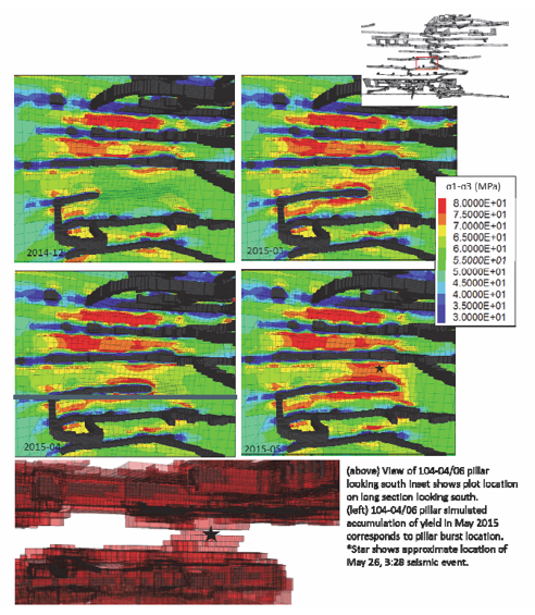
Figure: Evolution of numerically predicted stresses leading up to the MN3.2 event and numerically predicted pillar yield (Kalenchuk et al. 2017)
Some sites have sophisticated mine scale models that are updated and for which the calibration is improved from time to time. Such models provide a good opportunity to investigate what conditions lead up to large events or rockbursts. They also provide a good opportunity to back calculate parameter levels which can be used as values to flag possible adverse behaviour when using such models in forecast modelling.
Detailed forensic models are also run to obtain a better understanding of the mechanisms driving large events (Counter 2014), as shown in the figure below.
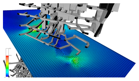
Figure: Forensic 3D elasto plastic model of a Mn3.9 seismic event. The slip surface is defined by major change in vector orientation and magnitude in the centre of the image. Local effect of unclamping in the foot wall caused by mining of a stope in the satallite lense (Counter 2014)
5.3 Forecast modelling
5.3.1 Standard
Some standard modelling approaches with established correlations and back calculated trigger values are used in forecast modelling to flag future adverse scenarios. For example, correlation of high mining induced stress/strength ratio and elevated seismicity with back calculated trigger levels are used to forecast when and where in the mine life stress conditions leading to adverse seismicity is expected to occur. Similar forecast models are performed with other parameters mentioned in Section 5.1.1.
5.3.2 Advanced
Forecast modelling using mine-wide calibrated elasto-plastic modelling, as shown in the following figure, or Salamon-Linkov modelling is performed at some sites. Considerable time and effort is invested in these models as they need to periodically be updated and re-calibrated as new information becomes available.
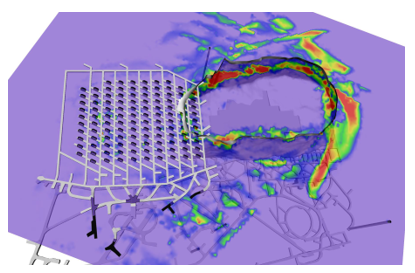
Figure: Contours of plastic shear strain from elasto–plastic modeling with strain-softening material behaviour. Red approximates a jump in damage from minor to moderate, moderate to significant, or significant to very significant